


")
Misalignment between physical progress and financial reporting frequently derails stable construction projects. Under the ASC 606 standard, recognized revenue relies on the cost-to-cost approach, meaning 4-6 week shipping delays do not just affect the schedule—they stall financial liquidity.
This article outlines how to calculate the Percentage of Completion (PoC) for accurate billing. We examine how to synchronize 42-micron acero galvanizado procurement with Make-to-Stock inventory cycles and manage the 2026 Chinese New Year supply chain disruption.

How to Calculate Timeline vs. Revenue for Your Stable Project?
For estable projects, the most accurate calculation method is the Percentage of Completion (PoC) using the cost-to-cost approach. Under the ASC 606 standard, you calculate revenue by dividing costs incurred to date by the estimated total costs. For example, if $500,000 of a $1,000,000 budget is spent, 50% of the total contract value is recognized immediately, linking financial health directly to physical progress.
The Percentage of Completion (PoC) Framework
Most construction and manufacturing projects utilize the ASC 606 standard to determine when revenue counts as earned. This framework moves away from simply billing when the job is done and instead recognizes value as it is created. Think of it like a progress bar on a file download; even if the download isn’t finished, the bar shows exactly how much data has been successfully transferred.
This method distinguishes between two types of recognition. Over-time recognition occurs when the customer benefits from the work as it happens, which is common in long-term builds. Point-in-time recognition happens only when the asset is fully handed over. To use the over-time method effectively, you must continuously track costs to validate timeline progress rather than waiting for the project conclusion.
The core formula is simple. You calculate the revenue to recognize by multiplying the percentage of the project that is complete by the total contract value.
Calculating Progress: The Cost-to-Cost Approach
The most objective way to measure how far along a project is involves following the money. This is known as the cost-to-cost approach. It assumes that the money you have spent on materials and labor directly correlates to the physical progress of the stable build.
You find your Percentage of Completion (POC) by dividing the costs incurred to date by the total estimated costs for the project. Once you have this percentage, you can determine your gross profit by taking the recognized revenue and subtracting the costs you have already paid.
| Calculation Step | Formula / Concept | Example Values |
|---|---|---|
| Step 1: Determine Progress | (Costs Incurred ÷ Total Est. Costs) × 100 | ($500k ÷ $1M) = 50% |
| Step 2: Recognize Revenue | Progress % × Total Contract Value | 50% × $2,000,000 = $1,000,000 |
| Step 3: Calculate Profit | Recognized Revenue – Costs Incurred | $1M – $500k = $500,000 |
Input vs. Output Measurement Methods
When tracking a timeline, you can measure what goes into the project or what comes out of it. Input methods focus on the effort expended. This includes tracking labor hours, machine operating time, or the quantity of materials consumed. This is useful for tasks that are uniform and repetitive.
Output methods measure the results achieved. This looks at physical milestones, such as laying the foundation, installing frames, or completing a specific number of units. Output methods often align better with client billing cycles because they represent tangible progress the client can see. However, input methods are generally better for tracking internal efficiency and cost control.
How DB Stable Optimizes Project Timelines
We utilize specific manufacturing and material choices to stabilize the variables in the cost-to-cost calculation. By focusing on prefabricated components, we reduce the variance in on-site input hours. Manufacturing components in a controlled factory environment stabilizes the labor cost ratio, making timeline predictions more accurate.
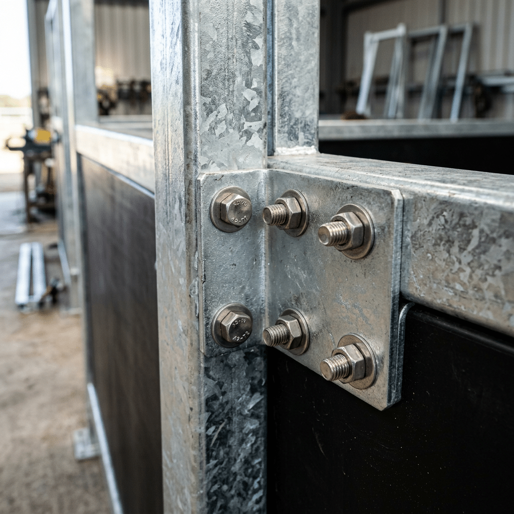
Material consistency also plays a role in predictable revenue recognition. We use hot-dip galvanized steel with a coating of 42 microns. Think of this as a heavy-duty, permanent shield that prevents rust for over a decade. This durability, combined with 10mm HDPE boards, reduces the risk of material waste or damage during transit, which can throw off cost estimates. Since 2013, our direct factory shipping ensures predictable delivery, allowing for accurate point-in-time revenue recognition. Additionally, professional guidance during the installation phase minimizes labor hour variances, keeping the project on the calculated timeline.
Step 1: Planning the Production Phase and Lead Times?
Lead time is the total duration between order placement and delivery completion. It is not a single event but a composite of five measurable elements: manufacturing, setup, transport, administrative tasks, and waiting time. Effective planning requires decomposing these stages to synchronize demand with capacity using backward scheduling.
Deconstructing the 5-Element Framework
To accurately plan production, managers must break down the total lead time into smaller, visible parts. This is similar to analyzing a relay race where every baton pass and running segment counts toward the final time. Gaining visibility into these specific components allows planners to identify exactly where delays occur.
- Waiting and Storage Time: This period historically consumes the largest share of the total lead time. It refers to the time materials sit idle between active processing steps, often exceeding the time spent actually manufacturing the product.
- Set-up and Administrative Time: This includes non-production activities that are essential but do not directly create the product. It covers order processing tasks and machine changeovers, which must be tracked alongside the physical work.
- Manufacturing and Transport: These are the active phases of creating and moving the product. Optimization strategies, such as the Single-Minute Exchange of Die (SMED), frequently target these areas to speed up the physical creation process.
Formulas and Variability: MTO vs. MTS
Calculating lead time requires a strict formula to ensure consistency. The standard calculation is the End of Production Date minus the Start of Production Date. For example, if an order begins on September 1 and finishes on September 10, the calculated lead time is 9 days. However, the scope of this calculation changes depending on the production model used.
- Make-to-Stock (MTS): ✅ Measured in days or weeks. The clock starts when the order is confirmed and stops when the truck departs. This model relies on having finished goods ready for immediate shipment.
- Make-to-Order (MTO): ✅ Often extends to months. This timeline encompasses the full procurement of raw materials and the manufacturing phases required for complex, custom products.
Critical Planning Constraints and Methodologies
Effective scheduling systems rely on accurate data to function correctly. Master Production Scheduling (MPS) uses lead time as a primary input to synchronize anticipated customer demand with the available labor and machine capacity. This ensures that the factory does not promise more than it can deliver within a specific timeframe.
- Constraint Variables: Planners must account for downtime data, such as maintenance and machine changeovers, as well as supplier limitations. Ignoring these factors leads to machine tool inactivity and production bottlenecks.
- Just-in-Time (JIT) Integration: Accurate lead time data allows production to trigger based on actual demand rather than forecasts. This reduces the overhead costs associated with storing excess inventory.
How DB Stable Optimizes Lead Times for Exports
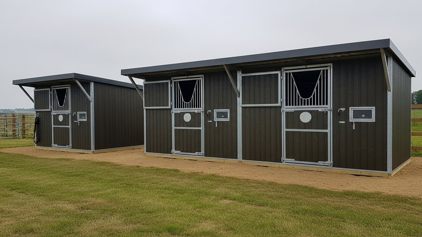
DB Stable applies these planning principles to the manufacturing of portable caballo stables, specifically for the Australian and New Zealand markets. By adopting a prefabricated manufacturing model, the company reduces the variability often found in custom on-site construction.
- Prefabricated Efficiency: Using modular components, such as the “9 Parts Stable Panel,” allows for standardized production. This reduces the manufacturing variable compared to building diseños personalizados from scratch.
- Logistics Synchronization: For exports to Australia and New Zealand, transport time is a fixed constraint. The planning team manages this through precise backward scheduling to ensure containers arrive on schedule.
- Inventory Readiness: By maintaining a stock of standard components like hot-dip galvanized frames and HDPE boards, DB Stable shifts its timeline closer to a Make-to-Stock model. This hybrid approach enables faster delivery than typical custom fabrication.

Step 2: Managing Shipping and Customs Buffers?
Shipping buffers are financial reserves (typically 10-50%) added to freight costs to absorb variances like fuel surcharges or dimensional weight, whereas customs buffers are schedule contingencies added to lead times for inspection delays. Effective management requires understanding that multiple shipping buffers compound mathematically rather than adding up simply.
Distinguishing Financial Costs from Schedule Contingencies
Successful logistics planning requires separating money problems from time problems. Shipping buffers act as financial insurance, while customs buffers act as schedule insurance. Understanding this distinction prevents budget overruns and missed deadlines.
- Shipping Buffers (Finance): These are extra funds set aside to cover cost spikes. They handle risks like rising fuel prices, currency exchange shifts, and dimensional weight charges where a package is priced by volume rather than actual weight.
- Customs Buffers (Time): These are extra days added to the schedule. They account for the time goods sit in holding while paperwork is verified or if a surprise inspection occurs.
- Integrated Planning: You must calculate cost adjustments for the finance department while simultaneously adding time contingencies to the delivery date for the operations team.
The Mathematics of Shipping Buffer Stacking
When applying financial buffers, the math is often multiplicative, not additive. If you simply add percentages together, you might underestimate the final cost. This is similar to how compound interest works in a bank account.
- Buffer Types: Adjustments happen at the Carrier level, which affects every shipment sent through that company, or at the Service level, which only affects specific modes like express air freight.
- Calculation Logic: Buffers stack on top of each other. If you have a $30 base rate, add a 10% carrier buffer ($33 total), and then add a 15% service buffer to that new total, the final cost is $37.95.
- Standard Variances: Planners often add 10% for standard shipping risks or up to 50% for dimensional weight variances. Fixed amounts, such as adding a flat $3 fee to a base rate, are also common.
Customs Compliance Pillars and Storage Constraints
Clearing customs without delays depends on strict adherence to rules. Think of this process as a three-legged stool; if one leg is missing, the shipment falls over and gets stuck at the border.
- Three Pillars of Compliance: Success relies on accurate documentation, correct HTS classification (the specific code that identifies your product), and following all import regulations.
- Storage Flexibility: If delays happen, goods held in U.S. customs warehouses can stay there for up to 5 years without duties or taxes being applied. This acts as a strategic waiting room for inventory.
- Risk Mitigation: Conducting risk assessments before the ship leaves the factory helps spot potential paperwork errors early.
How DB Stable Streamlines Delivery Timelines
For companies importing infrastructure like portable cuadras de caballos, navigating these buffers is critical. DB Stable utilizes its status as a direct factory to manage these variables effectively for clients in Australia and New Zealand.
- Document Expertise: The team manages export documentation internally, ensuring compliance with strict biosecurity and import regulations to prevent customs friction.
- Customer Experience: Clients frequently report that orders arrive in record time, which indicates that schedule buffers are managed efficiently.
- Factory Coordination: Operating since 2013, the factory coordinates production buffers with shipping windows. This helps maintain the lowest price promise by avoiding unnecessary storage fees or rush charges.
Engineered for Safety and Durability Worldwide
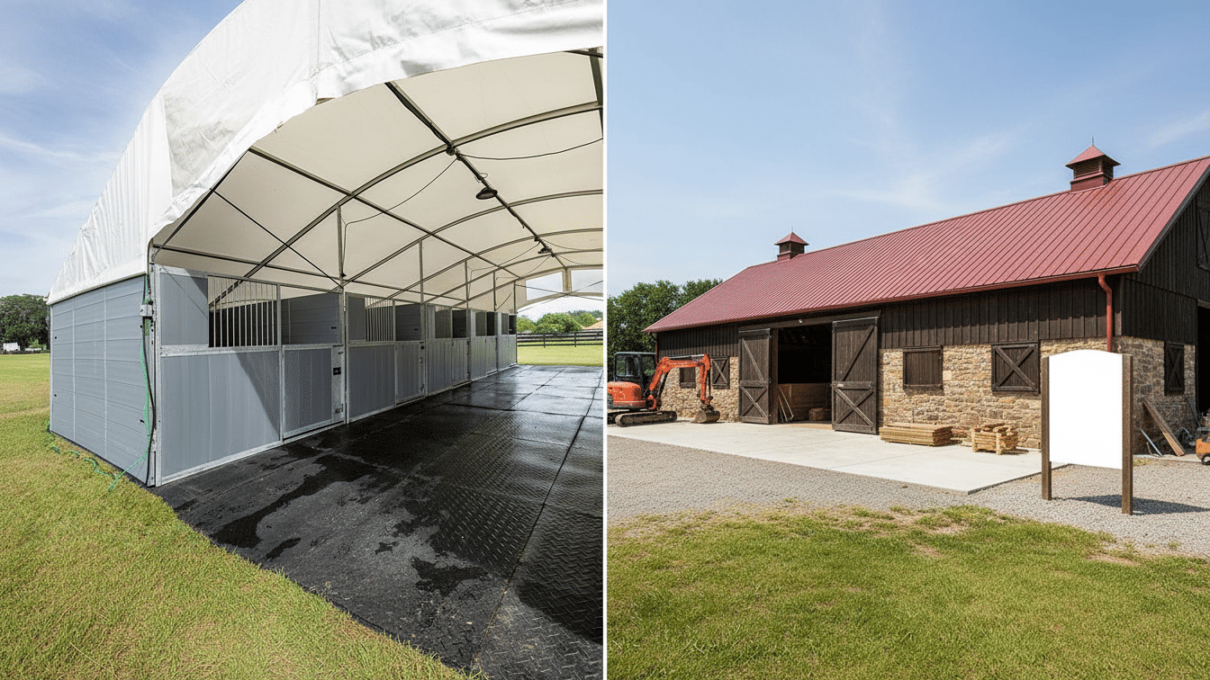
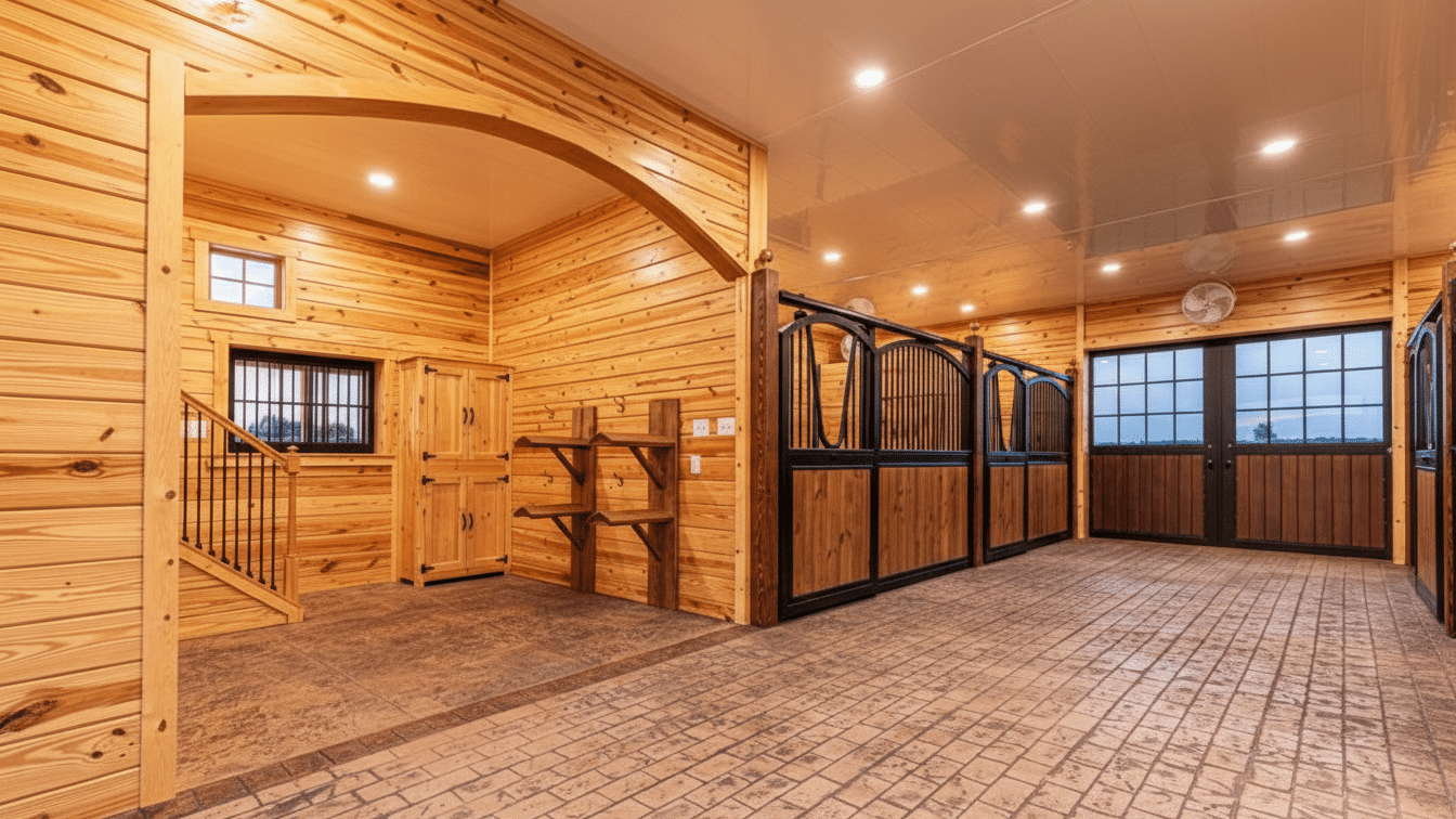
Protect your horses with precision-engineered establos diseñados to withstand extreme temperatures and weather conditions. Our modular, rust-resistant steel frameworks offer rapid installation and meet international normas de seguridad across Australia, Europe, and the USA.

Troubleshooting: Handling Delays During Chinese New Year?
Chinese New Year 2026 creates a supply chain freeze spanning 4–6 weeks, far exceeding the official 5-day holiday window. This disruption operates in three phases: a pre-holiday production rush causing quality risks, a total manufacturing halt starting mid-February, and a slow post-holiday recovery where factories struggle with labor shortages.
The Anatomy of the 4-6 Week Disruption
Most buyers assume the holiday is a simple one-week pause, similar to Western holidays. However, in Chinese manufacturing, the impact functions more like a complete seasonal shutdown followed by a reboot. The disruption begins weeks before the official dates and lingers long after factories reopen.
- Phase 1: Pre-Holiday Crunch (1–2 Weeks Prior): Workers often leave early to travel home, leveraging accrued overtime. This creates a production bottleneck where remaining staff rush to finish orders, which can lead to quality deviations if not monitored.
- Phase 2: The Shutdown (2–4 Weeks): Manufacturing across China and Taiwan halts completely. In 2026, the extended closure window runs from February 13–22 (a 10-day minimum), though many facilities remain closed longer to wait for workforce returns.
- Phase 3: The Slow Recovery (2–3 Weeks Post-Holiday): Operations lag as factories attempt to rehire staff. Data indicates approximately one-third of workers do not return to their jobs after the holiday, forcing factories to hire and train inexperienced replacements.
2026 Critical Dates and Cost Implications
Understanding the specific calendar for the 2026 season is essential for financial planning. The disruption affects not just production lines but also logistics networks, causing shipping delays and increased costs due to high demand.
- Official Holiday Window: February 16–20, 2026. Despite this short official window, the total supply chain disruption extends up to 6 weeks.
- Logistics Lag: Port and customs processing often experience extended lead times of 4–6 weeks even after shipping resumes, as they work through the accumulated backlog.
- Cost Surcharges: Carriers historically implement peak season surcharges during the pre-holiday rush. Historical data shows increases, such as UPS Asia-to-U.S. rates rising around $0.50/lb.
- Taiwan vs. China: While Taiwan factories may close for a shorter minimum of 7 days, the regional logistics network remains congested, affecting shipments from both areas.
Mitigation Strategy: The 6-Month Forecasting Rule
To prevent stockouts during this period, inventory planning must shift from a standard timeline to a proactive forecast model. The goal is to secure production slots before the pre-holiday rush compromises quality.
- ✅ The September/October Rule: Discuss orders intended for March or April delivery by September or October. This accounts for the full disruption cycle and ensures your spot in the production queue.
- ✅ Avoid January Rush Orders: Placing last-minute orders in early January increases exposure to quality failures. Factories are rushing to clear backlogs before the February 13 shutdown, which is when mistakes are most likely to occur.
- ✅ Buffer Inventory: Account for the post-holiday labor attrition rate. With up to 30% staff turnover, late March is a secondary risk period for control de calidad as new workers learn the ropes.
How DB Stable Manages Production Timelines
At DB Stable, we implement strict timeline management to protect our Australian and New Zealand clients from these seasonal fluctuations. Our process ensures that material quality remains consistent regardless of the time of year.
- Proactive Planning: We utilize the pre-holiday months to secure high-quality materials, specifically hot-dip galvanized steel with a 42-micron coating. This ensures that raw material shortages do not compound holiday delays.
- Customer Communication: Our project management team provides realistic timelines rather than optimistic estimates. We avoid the trap of over-promising, ensuring you know exactly when your stables will arrive.
- Quality Consistency: By avoiding the pre-holiday rush production trap, we maintain the integrity of critical components. This includes ensuring correct weld penetration on 6mm steel plates and proper formulation of UV-resistant HDPE boards, which requires precise temperature control during manufacturing.
Preguntas frecuentes
What is the typical lead time for ordering 20 stalls?
Standard industrial equipment typically requires an 8 to 16-week lead time depending on inventory levels. If you require engineered-to-order or highly customized stable projects, the timeline extends to 16 to 52 weeks. Professional planners calculate the lead time by taking the desired delivery date and subtracting the order date.
How does the CNY exchange rate and tariffs affect stable orders?
Reciprocal tariff rates reaching 145 percent are the primary numeric driver of order cost instability between the U.S. and China as of 2025. Additionally, profits for Chinese manufacturers have dropped 30 percent from 2021 to June 2025, forcing some factories to constrain capacity or raise prices. Volatility in the Yuan often correlates with logistics delays as central banks intervene to stabilize exchange rates.
Why are stable shipments frequently delayed?
Documentation errors, such as incorrect addresses or missing certificates, are a high-severity but controllable cause of delays. Port congestion also creates significant bottlenecks. Industry data shows that unloading a single vessel with 20,000 containers requires 3,000 people working for 3 days. Other unpredictable factors include physical roadblocks, mechanical failures, and extreme weather events.
When should I order stables for a summer build?
Construction principles define long-lead items as anything requiring four weeks or more, meaning they must be identified and ordered immediately during the planning phase. Standard construction materials currently face lead time ranges of 8 to 20 weeks. Waiting until spring to order often results in missing the summer construction window due to these accumulated delays.
How does DB Stable minimize lead time risks?
DB Stable operates with direct factory control, having managed production internally since 2013 to mitigate manufacturer capacity issues. The portable design utilizes hot-dip galvanized steel for prefabricated efficiency, allowing for faster deployment compared to traditional construction methods. Clients in Australia and New Zealand report that orders are delivered in record time by leveraging established shipping routes.
Reflexiones finales
The 2026 Chinese New Year disruption isn’t just a calendar event; it is a six-week supply chain freeze that threatens project viability. Waiting until January to finalize orders guarantees exposure to quality risks, labor shortages, and inevitable shipping surcharges.
Securing production slots before October bypasses the pre-holiday quality crunch and locks in current material rates. By stabilizing these variables early with DB Stable, you protect your capital and ensure your facility generates revenue while competitors are still waiting at the port.


0 comentarios